College Admissions, Part 1
Homework 12
College Admissions: From the College’s View
All of you have quite recently gone through the stressful process of figuring out which college to attend. You most likely selected colleges you thought might be a good fit, sent off applications, heard back from them, and then weighed your options. Those around you probably emphasized what an important decision this is for you and for your future.
Colleges see this process from an entirely different point of view. A college needs students to enroll first of all in order to collect enough tuition revenues in order to keep the lights on, the faculty paid, and, in the case Villanova, purchase TWO campuses. Almost all private colleges receive most of their revenues from tuition, and public colleges receive about equal amounts of funding from tuition and state funds, with state funds based on how many students they enroll. Second, colleges want to enroll certain types of students; colleges base their reputation on which students enroll, with greater prestige associated with enrolling students with better demonstrated academic qualifications. The job of enrolling a class that provides enough revenue AND has certain characteristics falls to the Enrollment Management office on a campus. This office typically includes the admissions office as well as the financial aid office.
The College Admissions “Funnel”
The admissions funnel is a well-established metaphor for understanding the enrollment process from the college’s perspective. It begins with colleges identifying prospective students: those who might be interested in enrolling. This proceeds to “interested” students, who engage with the college via registering on the college website, sending test scores, visiting campus, or requesting other information. Some portion of these interested students will then apply. Applicants are then considered, and admissions decisions are made. From this group of admitted students a certain proportion will actually enroll. Here’s data from Villanova on their enrollment funnel.
Each stage in this process involves modeling and prediction: how can we predict which prospective students will end up being interested students? How many interested students will turn into applicants? And, most importantly, how many admitted students will actually show up in the fall?
Colleges aren’t powerless in this process. Instead, they execute a careful strategy to intervene at each stage to get both the number and type of students they want to convert to the next stage. These are the core functions of enrollment management. Why did you receive so many emails, brochures and maybe even text messages? Some model somewhere said that the intervention could convert you from a prospect to an interest, or from an interest to an applicant.
We’re going to focus on the very last step: from admitted students to what’s called a yield: a student who actually shows up and sits down for classes in the fall.
The stakes are large: if too few students show up, then the institutions will not have enough revenues to operate. If too many show up the institution will not have capacity for all of them. On top of this, enrollment managers are also tasked with the combined goals of increasing academic prestige (usually through test scores and GPA) and increasing the socioeconomic diversity of the entering class. As we’ll see, these are not easy tasks.
The Data
We’re going to be using a dataset that was constructed to resemble a typical admissions dataset. To be clear: this is not real data, but instead is based on the relationships we see in actual datasets. Using real data in this case would be a violation of privacy.
library(tidyverse)
library(scales)ad<-read_rds("https://github.com/rweldzius/PSC4175/raw/main/static/data/admit_data.rds")%>%ungroup()Codebook for admit_data.rds:
| Variable Name | Description |
| ID | Student id |
| income | Family income (AGI) |
| sat | SAT/ACT score (ACT scores converted to SAT scale) |
| gpa | HS GPA, four point scale |
| visit | Did student visit campus? |
| legacy | Did student parent go to this college? |
| registered | Did student register on the website? |
| sent_scores | Did student send scores prior to applying? |
| distance | Distance from student home address to campus |
| tuition | Stated tuition: $45,000 |
| need_aid | Need-based aid offered |
| merit_aid | Merit-based aid offered |
| net_price | Net Price: Tuition less aid received |
| yield | Student enrolled in classes in fall after admission |
The Basics
## How many admitted students enroll?
ad%>%summarize(`Yield Rate`=percent(mean(yield)))
## Yield Rate
## 1 68%## Just for enrolled students
ad%>%filter(yield==1)%>%summarize(
`Average SAT Score`=number(mean(sat),accuracy=1,big.mark=""),
`Average GPA`=number(mean(gpa),accuracy = 1.11),
`Tuition`=dollar(mean(tuition)),
`Average Net Price`=dollar(mean(net_price),accuracy = 1 ),
`Total Tuition Revenues`=dollar(sum(net_price)),
`Total 1st Year Enrollment`=comma(n(),big.mark=",")) ## Average SAT Score Average GPA Tuition Average Net Price
## 1 1226 3.33 $45,000 $20,924
## Total Tuition Revenues Total 1st Year Enrollment
## 1 $30,674,149 1,466So, a few things stand out right away, all of which are pretty common among private colleges. First, this is a moderately selective institution, with an average GPA of 3.33 (unweighted) and an average SAT of about 1200 (about a 25 on the ACT). The average net price is MUCH less than tuition, indicating that the campus is discounting heavily. Total revenues from tuition are about 30 million.
The Case
We’ve been hired as the data science team for a liberal arts college (this is a real thing).
The college president and the board of trustees have two strategic goals:
- Increase the average SAT score to 1300
- Admit at least 200 more students with incomes less than $50,000
Here’s the rub: they want to do this without allowing tuition revenues to drop below $30 million and without changing the size of the entering class, which should be about 1,500 students (plus or minus 50, nobody minds sleeping in Falvey, right?).
What we need to do is to figure out which students are most and least likely to enroll. We can then target our financial aid strategy to improve yield rates among certain groups.
This is a well-known problem known as price discrimination, which is applied in many industries, including airlines, hotels, and software. The idea is to charge the customers who are most willing/able to pay the most, while charging the customers who are least willing/able to pay the least.
To solve our problem we need to do the following:
- Come up with a prediction algorithm that accurately establishes the relationship between student characteristics and the probability of attendance
- Adjust policies in order to target those students who we want to attend, thereby increasing their probability of attendance.
Current Institutional Policies
Essentially every private college engages heavily in tuition discounting. This has two basic forms: need-based aid and merit-based aid. Need-based aid is provided on the basis of income, typically with some kind of income cap. Merit-based aid is based on demonstrated academic qualifications, again usually with some kind of minimum. Here’s this institution’s current policies.
The institution is currently awarding need-based aid for families making less than $100,0000 on the following formula:
\(need_{aid}=500+(income/1000-100)*-425\)
Translated, this means for every $1,000 the family makes less than $100,000 the student receives an additional 425 dollars. So for a family making $50,000, need-based aid will be \(500+(50,000/1000-100)*-425= 500+ (-50*-425)\)=$21,750. Need based aid is capped at total tuition.
ad%>%
  ggplot(aes(x=income,y=need_aid))+
  geom_point()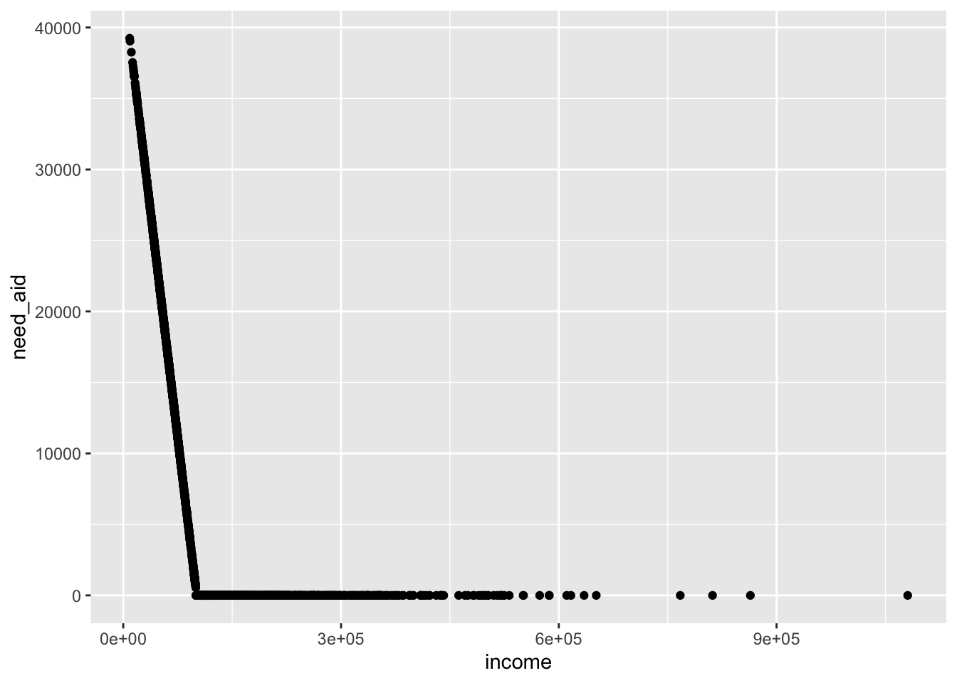
The institution is currently awarding merit-based aid for students with SAT scores above 1250 on the following formula:
\(merit_{aid}=5000+(sat/100*250)\)
Translated, this means that for every 10 points in SAT scores above 1250, the student will receive an additional $1,500. So for a student with 1400 SAT, merit based aid will be : \(5000+ (1400/10 *250)= 500+(140*250)\)
ad%>%
  ggplot(aes(x=sat,y=merit_aid))+
  geom_point()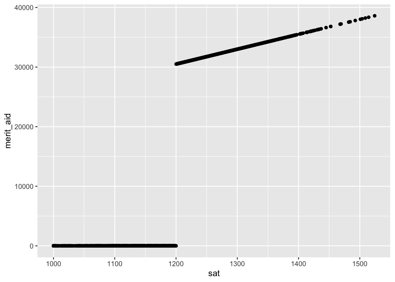
As with need-based aid, merit-based aid is capped by total tuition.
Classification
Our core prediction problem is classification. There are two groups of individuals that constitute our outcome: those who attended and those who did not. In data science, predicting group membership is known as a classification problem. It occurs whenever the outcome is a set of discrete groupings. We’ll be working with the simplest type of classification problem, which has just two groups, but these problems can have multiple groups, essentially categorical variables.
Probability of Attendance
Remember: the mean of a binary variable is the same thing as the proportion of the sample with that characteristic. So, the mean of yield is the same thing as the proportion of admitted students who attend, or the probability of attendance.
ad%>%summarize(pr_attend=mean(yield))## pr_attend
## 1 0.6818605Conditional Means
Let’s go back to our first algorithm for prediction: conditional means. Let’s start with the variable legacy which indicates whether or not the student has a parent who attended the same institution:
ad%>%
  group_by(legacy)%>%
  summarize(pr_attend=mean(yield))
## # A tibble: 2 × 2
## legacy pr_attend
## <dbl> <dbl>
## 1 0 0.641
## 2 1 0.780That’s a big difference! Legacy students are abut 14 percentage points more likely to yield than non-legacies.
Next, let’s look at SAT scores. This is a continuous variable, so we need to first break it up into a smaller number of groups. Let’s look at yield rates by quintile of SAT scores among admitted students:
ad%>%
  mutate(sat_quintile=ntile(sat,n=5))%>%
  group_by(sat_quintile)%>%
  summarize(min_sat=min(sat),
  pr_attend=mean(yield))
## # A tibble: 5 × 3
## sat_quintile min_sat pr_attend
## <int> <dbl> <dbl>
## 1 1 1000 0.440
## 2 2 1114. 0.533
## 3 3 1173. 0.691
## 4 4 1227. 0.828
## 5 5 1285. 0.919So, it looks like yield steadily increases with SAT scores– a good sign for the institution as it seeks to increase SAT scores.
Quick Exercise 1 calculate yield by quintiles of net price: what do you see?
ad%>%
  mutate(...)%>%
  group_by(... = )%>%
  summarize(amount=min(...),
            pr_attend=mean(...))
## Error in group_by(., ... = ): '...' used in an incorrect contextCombining Conditional Means
Let’s look at yield rates by both sat quintile and legacy status. What type of plot do you think we’ll use? Remember from the lectures on multivariate visualization. If you have Categorical X Categorical X Continuous, then use a tile plot!
ad%>%
  mutate(sat_decile=ntile(sat,n=10))%>%
  group_by(sat_decile,legacy)%>%
  summarize(min_sat=min(sat),
  pr_attend=mean(yield))%>%
  ggplot(aes(y=as_factor(sat_decile),x=as_factor(legacy),fill=pr_attend))+
  geom_tile()+
  scale_fill_viridis_c()+
  ylab("SAT Score Decile")+xlab("Legacy Status")
## `summarise()` has grouped output by 'sat_decile'. You can override using the
## `.groups` argument.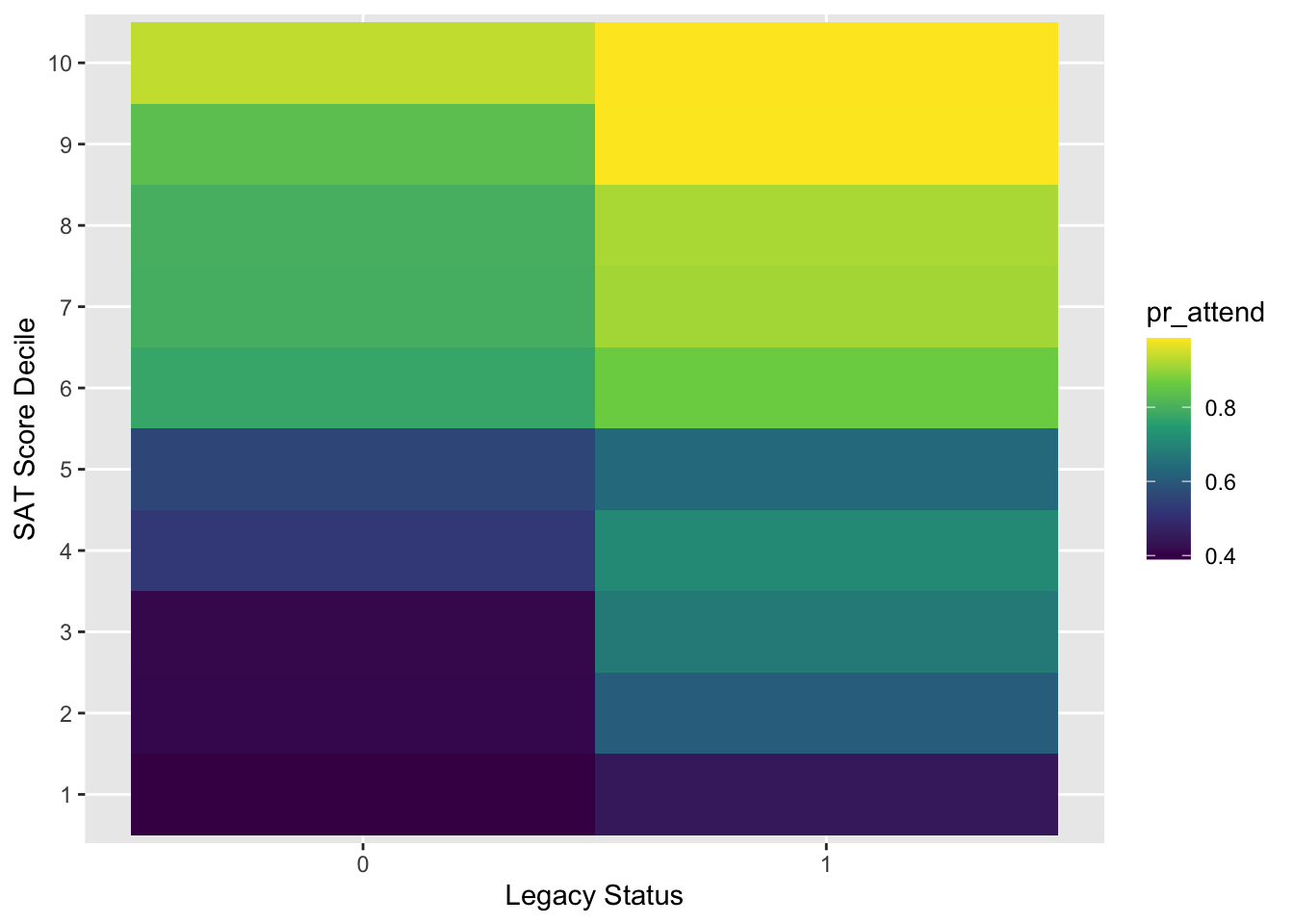
Predictions based on conditional means
We can use this simple method to make predictions.
ad<-ad%>%
  mutate(sat_quintile=ntile(sat,n=10))%>%
  group_by(sat_quintile,legacy)%>%
  mutate(prob_attend=mean(yield))%>%
  mutate(pred_attend=ifelse(prob_attend>=.5,1,0))
Let’s compare this predicted with the actual:
ad%>%
  group_by(yield,pred_attend)%>%
  summarize(n())%>%
  rename(`Actually Attended`=yield,
         `Predicted to Attend`=pred_attend,
         `Number of Students`=`n()`)
## `summarise()` has grouped output by 'yield'. You can override using the
## `.groups` argument.## # A tibble: 4 × 3
## # Groups: Actually Attended [2]
## `Actually Attended` `Predicted to Attend` `Number of Students`
## <int> <dbl> <int>
## 1 0 0 304
## 2 0 1 380
## 3 1 0 210
## 4 1 1 1256Acccuracy of Conditional Means
ad%>%
  group_by(yield)%>%
  mutate(total_attend=n())%>%
  group_by(yield,pred_attend)%>%
  summarize(n(),`Actual Group`=mean(total_attend))%>%
  mutate(Proportion=`n()`/`Actual Group`)%>%
  rename(`Actually Attended`=yield,
         `Predicted to Attend`=pred_attend,
         `Number of Students`=`n()`)
## `summarise()` has grouped output by 'yield'. You can override using the
## `.groups` argument.## # A tibble: 4 × 5
## # Groups: Actually Attended [2]
## `Actually Attended` `Predicted to Attend` `Number of Students` `Actual Group`
## <int> <dbl> <int> <dbl>
## 1 0 0 304 684
## 2 0 1 380 684
## 3 1 0 210 1466
## 4 1 1 1256 1466
## # ℹ 1 more variable: Proportion <dbl>Here’s how to read this: There were 304 students that our algorithm said would not attend who didn’t attend. This means out of the 684 students who were admitted but did not attend, our algorithm correctly classified 44 percent. There were 380 students who our model said would not attend who actually showed up (or 56 percent).
On the other side, there were 210 students who our model said would not show up, who actually attended. And last, there were 1256 students who our model said would attend who actually did; we correctly classified 85 percent of actual attendees. The overall accuracy of our model ends up being (304+1256)/2150 or 73 percent.
Question: is this a good model?
Prediction via Linear Regression: Wrong, but Useful!
We can use our standard tool of linear regression to build a model and make predictions, with just a few adjustments. This will be wrong, but useful.
We’ll use the wrong model, a linear regression. Running a linear regression with a binary dependent variable is called a linear probability model, which ironically it is not.
We’ll use a formula that includes the variables we’ve used so far.
admit_formula<-as.formula("yield~sat+net_price+legacy")

ad_analysis <- ad %>%
  ungroup() %>%
  select(yield,sat,net_price,legacy) %>%
  drop_na()

m <- lm(formula = admit_formula,data = ad_analysis)
summary(m)
##
## Call:
## lm(formula = admit_formula, data = ad_analysis)
##
## Residuals:
## Min 1Q Median 3Q Max
## -1.1497 -0.3714 0.1338 0.3055 0.9392
##
## Coefficients:
## Estimate Std. Error t value Pr(>|t|)
## (Intercept) -2.981e+00 1.514e-01 -19.696 < 2e-16 ***
## sat 2.842e-03 1.173e-04 24.222 < 2e-16 ***
## net_price 1.052e-05 7.447e-07 14.122 < 2e-16 ***
## legacy 9.502e-02 1.954e-02 4.863 1.24e-06 ***
## ---
## Signif. codes: 0 '***' 0.001 '**' 0.01 '*' 0.05 '.' 0.1 ' ' 1
##
## Residual standard error: 0.409 on 2146 degrees of freedom
## Multiple R-squared: 0.2302, Adjusted R-squared: 0.2291
## F-statistic: 213.9 on 3 and 2146 DF, p-value: < 2.2e-16Question: What do we make of these coefficients
To evaluate our model, we traditionally have relied on RMSE. However, this is less appropriate when using a binary dependent variable. Instead, we want to think about accuracy. Let’s start by getting the predictions, as always.
ad_analysis <- ad_analysis %>%
  mutate(preds = predict(m)) %>%
  mutate(errors = yield - preds)
Let’s take a look at these predictions
ad_analysis %>% select(yield,preds)## # A tibble: 2,150 × 2
## yield preds
## <int> <dbl>
## 1 1 0.735
## 2 1 1.07
## 3 1 0.245
## 4 0 0.683
## 5 1 0.589
## 6 0 0.358
## 7 1 0.559
## 8 1 0.757
## 9 0 0.366
## 10 0 0.698
## # ℹ 2,140 more rowsSo these are probabilities. To complete the classification problem, we need to assign group labels to each case in the testing dataset. Let’s assume that a probability equal to or greater than .5 will be classified as a 1 and everything else as a 0.
ad_analysis<-ad_analysis%>%
  mutate(pred_attend=ifelse(preds>=.5,1,0))

ad_analysis%>%select(yield,preds,pred_attend)
## # A tibble: 2,150 × 3
## yield preds pred_attend
## <int> <dbl> <dbl>
## 1 1 0.735 1
## 2 1 1.07 1
## 3 1 0.245 0
## 4 0 0.683 1
## 5 1 0.589 1
## 6 0 0.358 0
## 7 1 0.559 1
## 8 1 0.757 1
## 9 0 0.366 0
## 10 0 0.698 1
## # ℹ 2,140 more rowsHere’s the problem with using a linear regression in this case: there’s no guarantee that the results will be on the probability scale. So, we can find cases where our model predicted probabilities below 0 or above 1. Of course, these just get labeled as 1 or 0.
ad_analysis%>%
  filter(preds>1|preds<0)%>%
  select(yield,preds,pred_attend)
## # A tibble: 128 × 3
## yield preds pred_attend
## <int> <dbl> <dbl>
## 1 1 1.07 1
## 2 1 1.06 1
## 3 1 1.02 1
## 4 1 1.10 1
## 5 1 1.03 1
## 6 1 1.12 1
## 7 1 1.18 1
## 8 1 1.49 1
## 9 1 1.15 1
## 10 1 1.11 1
## # ℹ 118 more rowsAccuracy of Linear Regression
ad_analysis%>%
  group_by(yield)%>%
  mutate(total_attend=n())%>%
  group_by(yield,pred_attend)%>%
  summarize(n(),`Actual Group`=mean(total_attend))%>%
  mutate(Proportion=`n()`/`Actual Group`)%>%
  rename(`Actually Attended`=yield,
         `Predicted to Attend`=pred_attend,
         `Number of Students`=`n()`)
## `summarise()` has grouped output by 'yield'. You can override using the
## `.groups` argument.## # A tibble: 4 × 5
## # Groups: Actually Attended [2]
## `Actually Attended` `Predicted to Attend` `Number of Students` `Actual Group`
## <int> <dbl> <int> <dbl>
## 1 0 0 282 684
## 2 0 1 402 684
## 3 1 0 113 1466
## 4 1 1 1353 1466
## # ℹ 1 more variable: Proportion <dbl>In this model, we correctly classified 282 out of 684 non-attendees or about 41 percent, and 1353 out of 1466 attendees or about 92 percent. The overall accuracy is (282+1353)/2150 or 76 percent. How are we doing?
Sensitivity
In the above table, the percent of 1s correctly identified is a measure known as sensitivity:
ad_analysis%>%
  group_by(yield)%>%
  mutate(total_attend=n())%>%
  group_by(yield,pred_attend)%>%
  summarize(n(),`Actual Group`=mean(total_attend))%>%
  mutate(Proportion=`n()`/`Actual Group`)%>%
  rename(`Actually Attended`=yield,
         `Predicted to Attend`=pred_attend,
         `Number of Students`=`n()`) %>%
  filter(`Actually Attended` == 1 & `Predicted to Attend` == 1)
## `summarise()` has grouped output by 'yield'. You can override using the
## `.groups` argument.## # A tibble: 1 × 5
## # Groups: Actually Attended [1]
## `Actually Attended` `Predicted to Attend` `Number of Students` `Actual Group`
## <int> <dbl> <int> <dbl>
## 1 1 1 1353 1466
## # ℹ 1 more variable: Proportion <dbl>Specificity
The percent of 0s correctly identified is a measure known as specificity
ad_analysis%>%
  group_by(yield)%>%
  mutate(total_attend=n())%>%
  group_by(yield,pred_attend)%>%
  summarize(n(),`Actual Group`=mean(total_attend))%>%
  mutate(Proportion=`n()`/`Actual Group`)%>%
  rename(`Actually Attended`=yield,
         `Predicted to Attend`=pred_attend,
         `Number of Students`=`n()`) %>%
  filter(`Actually Attended` == 0 & `Predicted to Attend` == 0)
## `summarise()` has grouped output by 'yield'. You can override using the
## `.groups` argument.## # A tibble: 1 × 5
## # Groups: Actually Attended [1]
## `Actually Attended` `Predicted to Attend` `Number of Students` `Actual Group`
## <int> <dbl> <int> <dbl>
## 1 0 0 282 684
## # ℹ 1 more variable: Proportion <dbl>Accuracy
ad_analysis%>%
  group_by(yield)%>%
  mutate(total_attend=n())%>%
  group_by(yield,pred_attend)%>%
  summarize(n(),`Actual Group`=mean(total_attend))%>%
  mutate(Proportion=`n()`/`Actual Group`)%>%
  rename(`Actually Attended`=yield,
         `Predicted to Attend`=pred_attend,
         `Number of Students`=`n()`) %>%
  filter(`Actually Attended` == `Predicted to Attend`) %>%
  ungroup() %>%
  summarise(Accuracy = sum(`Number of Students`) / sum(`Actual Group`))
## `summarise()` has grouped output by 'yield'. You can override using the
## `.groups` argument.## # A tibble: 1 × 1
## Accuracy
## <dbl>
## 1 0.760