Binary Predictors and Multiple Regression
Homework 11
Introduction
In this section we’re going to continue fitting regressions to the training data and testing the predictions against the testing data. We’ll include additional continuous variables. We’re also going to add some new elements. In particular, We’ll be using independent variables or predictor variables that are binary or categorical.
We’ll need the same libraries as last week:
library(tidyverse)
library(plotly)
library(scales)
And the same dataset, which includes data on movies released since 1980.
mv<-readRDS(url("https://github.com/rweldzius/PSC4175/raw/main/static/data/mv.Rds")) %>%
  filter(!is.na(budget))%>%
  mutate(log_gross=log(gross),
         log_budget = log(budget))%>%
  mutate(bechdel_bin=ifelse(bechdel_score==3,1,0))%>%
  mutate(bechdel_factor=recode_factor(bechdel_bin,
                                      `1`="Pass",
                                      `0`="Fail",
                                      ))
A Brief Digression: The Bechdel Test
The Bechdel test was first made famous by Alison Bechdel in 1985– Bechdel credited the idea to Liz Wallace and her reading of Virginia Woolf. It asks three questions about a movie:
- Does it have two women in it?
- Who talk to each other?
- About something other than a man?
The test sets an unbelievably low bar, and yet a remarkable number of movies don’t pass it. One excuse sometimes used by filmmakers is that movie audiences tend to be young and male, and so favor movies that don’t necessarily pass this test. However, a study by CAA and shift7 called this logic into question:
A study indicates that female-led movies make more money thatn those that are not.
Let’s see if we can replicate their results in this data. First of all, what proportion of these movies made since 2000 pass the Bechdel test?
mv%>%
  group_by(bechdel_bin)%>%
  count()
## # A tibble: 3 × 2
## # Groups: bechdel_bin [3]
## bechdel_bin n
## <dbl> <int>
## 1 0 873
## 2 1 1186
## 3 NA 1132A majority, but 873 (873!!) movies did not have two female characters that spoke to each other about anything other than a man.
Let’s see if the contention of movie execs about earning power holds up.
mv%>%
  mutate(budget_level=ntile(budget,n=5))%>%
  group_by(budget_level,bechdel_factor)%>%
  summarize(mean_gross=mean(gross,na.rm=TRUE))%>%
  drop_na()%>%
  ggplot(aes(x=budget_level,y=mean_gross,fill=bechdel_factor))+
  geom_col(position="dodge")+
  scale_y_continuous(labels=dollar_format())+
  ylab("Gross Earnings")+xlab("Size of Movie Budget")+
  scale_fill_discrete(name="Passed Bechdel Test")+
  theme_minimal()+
  theme(legend.position = "bottom")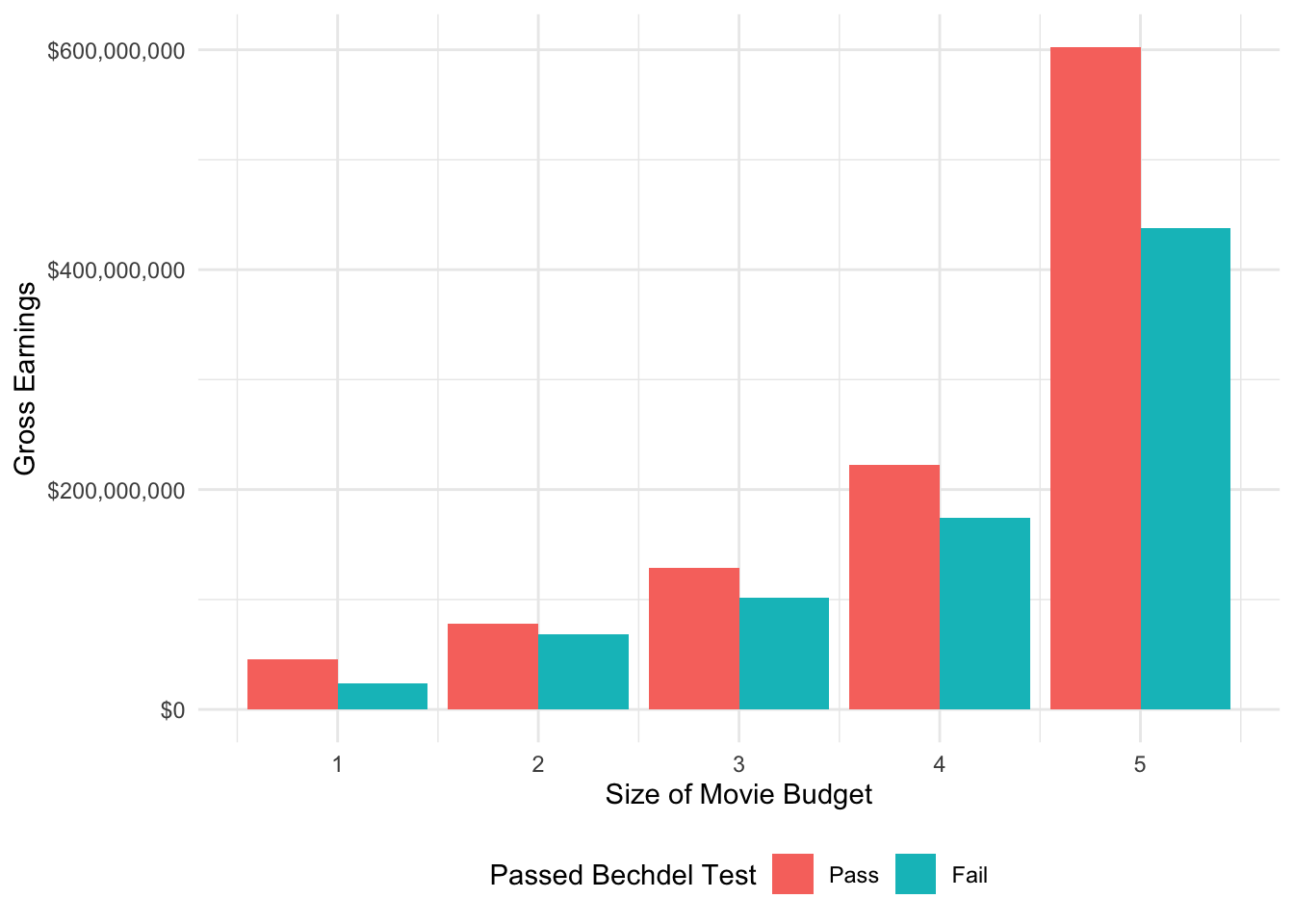
Nope. At every budget level, movies that pass the Bechdel test make more money, not less.
Regression with a binary variable
Let’s see if we can use regression to obtain a similar result. The next variable I want to include is the Bechdel variable, which is a binary variable set to “1” if the movie passes the Bechdel test.
mv%>%
  group_by(bechdel_bin)%>%
  summarize(count=n())%>%
  mutate(`Proportion`=count/sum(count))%>%
  arrange(-Proportion)
## # A tibble: 3 × 3
## bechdel_bin count Proportion
## <dbl> <int> <dbl>
## 1 1 1186 0.372
## 2 NA 1132 0.355
## 3 0 873 0.274Regression
Next, I add the variable bechdel_factor to the formula. Recall from the previous lecture that we ended with a multiple regression model in which we predicted gross by the budget and the IMDB score.
mBech <- lm(log_gross ~ log_budget + score + bechdel_factor,mv)
summary(mBech)
##
## Call:
## lm(formula = log_gross ~ log_budget + score + bechdel_factor,
## data = mv)
##
## Residuals:
## Min 1Q Median 3Q Max
## -8.6909 -0.4825 0.1423 0.6341 8.0510
##
## Coefficients:
## Estimate Std. Error t value Pr(>|t|)
## (Intercept) 0.47383 0.39162 1.210 0.226
## log_budget 0.92779 0.01955 47.464 < 2e-16 ***
## score 0.26226 0.02827 9.278 < 2e-16 ***
## bechdel_factorFail -0.21934 0.05160 -4.251 2.23e-05 ***
## ---
## Signif. codes: 0 '***' 0.001 '**' 0.01 '*' 0.05 '.' 0.1 ' ' 1
##
## Residual standard error: 1.143 on 2054 degrees of freedom
## (1133 observations deleted due to missingness)
## Multiple R-squared: 0.5303, Adjusted R-squared: 0.5296
## F-statistic: 772.9 on 3 and 2054 DF, p-value: < 2.2e-16The variable bechdel_factor is now added to our formula. Note that, because it is a binary categorical variable, we only have one value for it. This is because the regression is comparing a movie that fails the Bechdel test to one that passes it. Thus we can think of the coefficient -0.219 as the difference between a movie that passes and fails the test – i.e., movies that fail the test gross less than those that pass it. Note that this relationship holds even AFTER controlling for budget and IMDB score.
Calculating model fit with RMSE
Recall how to calculate the root mean square error (RMSE). We: 1. Estimate our model 2. Calculate predicted outcomes 3. Calculate errors (predicted - true values) 4. Square the errors 5. Take the average of the squared errors 6. Take the square root of this average
e <- resid(mBech)
se <- e^2
mse <- mean(se)
rmse <- sqrt(mse)
rmse
## [1] 1.141396But we don’t want to calculate this on the full data. Instead, we rely on cross validation to get a more accurate measure of our model’s fit. Also! Remember that we are interested in comparing how good our model performs with different combinations of predictors. Does the Bechdel data actually help us?
set.seed(123)
mvAnalysis <- mv %>%
  select(bechdel_factor,score,log_budget,log_gross) %>%
  drop_na()

cvRes <- NULL

for(i in 1:100) {
  inds <- sample(1:nrow(mvAnalysis),size = round(nrow(mvAnalysis)*.75),replace = F) # Set training to 75% of the data
  train <- mvAnalysis %>% slice(inds)
  test <- mvAnalysis %>% slice(-inds)

  # Three models of increasing complexity
  m1 <- lm(log_gross ~ log_budget,train)
  m2 <- lm(log_gross ~ log_budget + score,train)
  m3 <- lm(log_gross ~ log_budget + score + bechdel_factor,train)

  # Calculate RMSE for each
  cvRes <- test %>%
    mutate(pred1 = predict(m1,newdata = test),
           pred2 = predict(m2,newdata = test),
           pred3 = predict(m3,newdata = test)) %>%
    summarise(rmse1 = sqrt(mean((log_gross - pred1)^2,na.rm=T)),
              rmse2 = sqrt(mean((log_gross - pred2)^2,na.rm=T)),
              rmse3 = sqrt(mean((log_gross - pred3)^2,na.rm=T))) %>%
    mutate(cvIndex = i) %>%
    bind_rows(cvRes)

}

cvRes %>%
  select(-cvIndex) %>%
  summarise_all(mean) %>%
  gather(model,rmse) %>%
  ggplot(aes(x = rmse,y = reorder(model,rmse))) +
  geom_bar(stat = 'identity')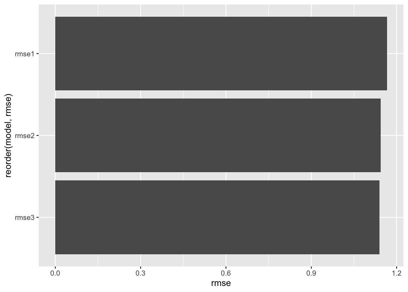
cvRes %>%
  select(-cvIndex) %>%
  gather(model,rmse) %>%
  ggplot(aes(x = rmse,fill = model)) +
  geom_density(alpha = .3)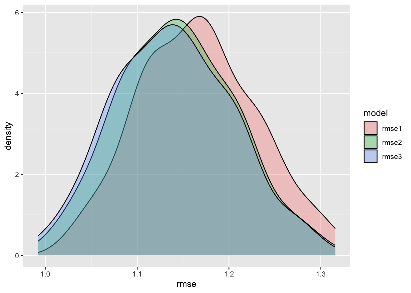
cvRes %>%
  summarise(diff12 = round(mean(rmse1 > rmse2),3),
            diff13 = round(mean(rmse1 > rmse3),3),
            diff23 = round(mean(rmse2 > rmse3),3)) %>%
  as.data.frame()
## diff12 diff13 diff23
## 1 1 1 0.87So we improve the model fit by adding the Bechdel test scores. We are 99.9% certain that model 2 is an improvement over model 1, 99.9% sure that model 3 is an improvement over model 1, and 87% sure that model 3 is an improvement over model 2.
Regression with a categorical variable
We can also include categorical variables (not just binary variables) in our model using much the same process. Let’s see if a movie’s MPAA Rating is related to its gross.
What numbers of movies have different ratings?
mv%>%
  group_by(rating)%>%
  count()
## # A tibble: 9 × 2
## # Groups: rating [9]
## rating n
## <chr> <int>
## 1 G 54
## 2 NC-17 6
## 3 Not Rated 37
## 4 PG 434
## 5 PG-13 1249
## 6 R 1392
## 7 TV-MA 2
## 8 Unrated 7
## 9 <NA> 10Regressing + Model Test
Let’s analyze!
summary(m2 <- lm(log_gross ~ log_budget + score + rating,mv))##
## Call:
## lm(formula = log_gross ~ log_budget + score + rating, data = mv)
##
## Residuals:
## Min 1Q Median 3Q Max
## -7.1259 -0.5786 0.1573 0.7163 8.0714
##
## Coefficients:
## Estimate Std. Error t value Pr(>|t|)
## (Intercept) 1.62557 0.39228 4.144 3.50e-05 ***
## log_budget 0.85421 0.01842 46.373 < 2e-16 ***
## score 0.33985 0.02256 15.064 < 2e-16 ***
## ratingNC-17 -1.18817 0.51972 -2.286 0.02231 *
## ratingNot Rated -2.33824 0.26865 -8.704 < 2e-16 ***
## ratingPG -0.24143 0.17397 -1.388 0.16530
## ratingPG-13 -0.43612 0.16768 -2.601 0.00934 **
## ratingR -0.93461 0.16874 -5.539 3.30e-08 ***
## ratingTV-MA -2.26996 0.86839 -2.614 0.00899 **
## ratingUnrated -2.36506 0.48738 -4.853 1.28e-06 ***
## ---
## Signif. codes: 0 '***' 0.001 '**' 0.01 '*' 0.05 '.' 0.1 ' ' 1
##
## Residual standard error: 1.205 on 3164 degrees of freedom
## (17 observations deleted due to missingness)
## Multiple R-squared: 0.5352, Adjusted R-squared: 0.5339
## F-statistic: 404.8 on 9 and 3164 DF, p-value: < 2.2e-16How to interpret this output? Again, we want to be aware of which category is not being included, which is the reference to the rest of the rating categories. As you can see, this is the “G” movie rating (i.e., general audiences). As we can see, G-rated movies earn more than EVERY OTHER TYPE OF MOVIE.
Note that we might want to drop certain rarely occurring categories. For example, we know from above that there are only 6 NC-17 movies, 2 TV-MA movies, and 7 Unrated movies. Furthermore, we can change the reference category to something different with the factor() command. Let’s do this now:
mvAnalysis <- mv %>%
  select(log_gross,log_budget,score,rating) %>%
  filter(!rating %in% c('NC-17','TV-MA','Unrated')) %>%
  drop_na() %>%
  mutate(rating = factor(rating,levels = c('R','PC-13','PG','G','Not Rated')))

summary(m3 <- lm(log_gross ~ log_budget + score + rating,mvAnalysis))
##
## Call:
## lm(formula = log_gross ~ log_budget + score + rating, data = mvAnalysis)
##
## Residuals:
## Min 1Q Median 3Q Max
## -6.8665 -0.6266 0.1777 0.7816 7.9003
##
## Coefficients:
## Estimate Std. Error t value Pr(>|t|)
## (Intercept) 0.99416 0.46538 2.136 0.0328 *
## log_budget 0.82891 0.02495 33.220 < 2e-16 ***
## score 0.35852 0.03220 11.136 < 2e-16 ***
## ratingPG 0.72476 0.07763 9.336 < 2e-16 ***
## ratingG 0.96838 0.18522 5.228 1.9e-07 ***
## ratingNot Rated -1.44571 0.23159 -6.242 5.3e-10 ***
## ---
## Signif. codes: 0 '***' 0.001 '**' 0.01 '*' 0.05 '.' 0.1 ' ' 1
##
## Residual standard error: 1.317 on 1904 degrees of freedom
## (1249 observations deleted due to missingness)
## Multiple R-squared: 0.5032, Adjusted R-squared: 0.5018
## F-statistic: 385.6 on 5 and 1904 DF, p-value: < 2.2e-16As we can see, every type of movie earns more than rated-R movies with the exception of Not Rated movies, which earn less.
Let’s evaluate RMSE again via cross validation.
cvRes2 <- NULL

for(i in 1:100) {
  inds <- sample(1:nrow(mvAnalysis),size = round(nrow(mvAnalysis)*.75),replace = F) # Set training to 75% of the data
  train <- mvAnalysis %>% slice(inds)
  test <- mvAnalysis %>% slice(-inds)

  # Three models of increasing complexity
  m1 <- lm(log_gross ~ log_budget,train)
  m2 <- lm(log_gross ~ log_budget + score,train)
  m3 <- lm(log_gross ~ log_budget + score + rating,train)

  # Calculate RMSE for each
  cvRes2 <- test %>%
    mutate(pred1 = predict(m1,newdata = test),
           pred2 = predict(m2,newdata = test),
           pred3 = predict(m3,newdata = test)) %>%
    summarise(rmse1 = sqrt(mean((log_gross - pred1)^2,na.rm=T)),
              rmse2 = sqrt(mean((log_gross - pred2)^2,na.rm=T)),
              rmse3 = sqrt(mean((log_gross - pred3)^2,na.rm=T))) %>%
    mutate(cvIndex = i) %>%
    bind_rows(cvRes2)

}

cvRes2 %>%
  select(-cvIndex) %>%
  summarise_all(mean) %>%
  gather(model,rmse) %>%
  ggplot(aes(x = rmse,y = reorder(model,rmse))) +
  geom_bar(stat = 'identity')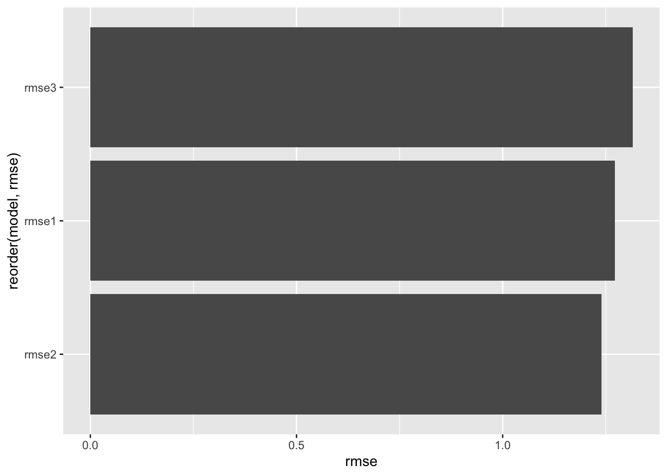
cvRes2 %>%
  select(-cvIndex) %>%
  gather(model,rmse) %>%
  ggplot(aes(x = rmse,fill = model)) +
  geom_density(alpha = .3)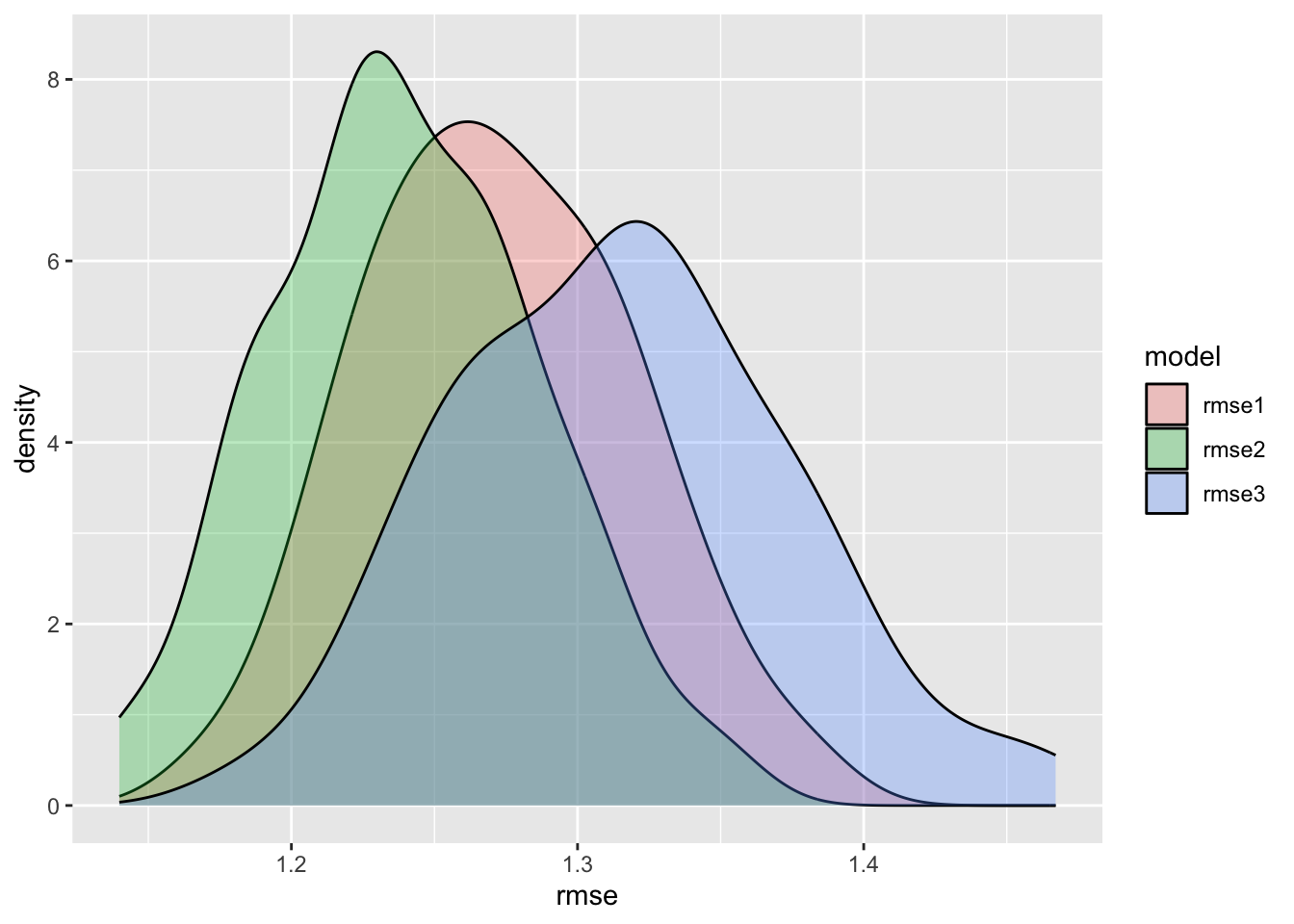
cvRes2 %>%
  summarise(diff12 = mean(rmse1 > rmse2),
            diff13 = mean(rmse1 > rmse3),
            diff23 = mean(rmse2 > rmse3))
## # A tibble: 1 × 3
## diff12 diff13 diff23
## <dbl> <dbl> <dbl>
## 1 1 0.07 0.01We are now finding that adding the rating reduces the fit of our model, as evidence by a higher RMSE! Why might this be the case?
Last Note
Remember that we need to carefully distinguish between categorical variables and continuous variables when including them in our models. If we’re using categorical variables we’ll need to pre-process the data in order to let the model know that these variables should be included as categorical variables, with an excluded reference category.
Research Exercise 1: Write a short plan for your final project. First, be sure to state what you are testing, what’s your data, and what do you hope to do/show with this data? Next, provide a timeline for completing these tasks using the rubric below. That’s it!
Write answer here about your project
Timeline for final project:
Week 11 (Nov. 10):
Week 12 (Nov. 17):
Week 13 (Nov. 24; includes Thanksgiving):
Week 14 (Dec. 1):
Week 15 (Dec. 8; presentations will begin):