Confidence and Uncertainty
Homework 7
Uncertainty
When we calculate a summary statistic in univariate statistics, we’re making a statement about what we can expect to see in other situations. If I say that the average height of a cedar tree is 75 feet, that gives an expectation for the average height we might calculate for any given sample of cedar trees. However, there’s more information that we need to communicate. It’s not just the summary measure– it’s also our level of uncertainty around that summary measure. Sure, the average height might be 75 feet, but does that mean in every sample we ever collect we’re always going to see an average of 75 feet?
Motivating Question
We’ll be working with data from every NBA player who was active during the 2018-19 season.
Here’s the data:
require(tidyverse)
nba<-read_rds("https://github.com/rweldzius/PSC4175/raw/main/static/data/nba_players_2018.Rds")
This data contains the following variables:
Codebook for NBA Data
| Name | Definition |
|---|---|
| namePlayer | Player name |
| idPlayer | Unique player id |
| slugSeason | Season start and end |
| numberPlayerSeason | Which season for this player |
| isRookie | Rookie season, true or false |
| slugTeam | Team short name |
| idTeam | Unique team id |
| gp | Games Played |
| gs | Games Started |
| fgm | Field goals made |
| fga | Field goals attempted |
| pctFG | Percent of field goals made |
| fg3m | 3 point field goals made |
| fg3a | 3 point field goals attempted |
| pctFG3 | Percent of 3 point field goals made |
| pctFT | Free Throw percentage |
| fg2m | 2 point field goals made |
| fg2a | 2 point field goals attempted |
| pctFG2 | Percent of 2 point field goals made |
| agePlayer | Player age |
| minutes | Minutes played |
| ftm | Free throws made |
| fta | Free throws attempted |
| oreb | Offensive rebounds |
| dreb | Defensive rebounds |
| treb | Total rebounds |
| ast | Assists |
| blk | Blocks |
| tov | Turnovers |
| pf | Personal fouls |
| pts | Total points |
| urlNBAAPI | Source url |
We might be interested in a variety of questions:
- Do certain colleges produce players that have more field goals? What about free throw percentage above a certain level? Are certain colleges in the east or the west more likely to produce higher scorers? How does this vary as a player has more seasons?
To answer these questions we need to look at the following variables:
- Field goals
- Free throw percentage above .25
- Colleges
- Player seasons
- Region
For me, I’m most curious if the Eastern or Western conferences have different styles of play. In particular, I want to know if one conference fouls more than the other.
Continuous by Categorical
Recall that there are two conference in the NBA, eastern and western. Let’s take a look at the variable that indicates which conference the player played in that season.
nba%>%select(idConference)%>%
  glimpse()
## Rows: 530
## Columns: 1
## $ idConference <int> 2, 2, 2, 2, 1, 1, 2, 1, 1, 2, 2, 1, 2, 1, 1, 1, 1, 2, 2, …It looks like conference is structured as numeric, but a “1” or a “2”. Because it’s best to have binary variables structured as “has the characteristic” or “doesn’t have the characteristic” we’re going to create a variable for western conference that’s set to 1 if the player was playing in the western conference and 0 if the player was not (this is the same as playing in the eastern conference).
nba<-nba%>%
  mutate(conference=ifelse(idConference==1,'West','East'))
Now that we’ve wrangled, let’s compare personal fouls among players in the east versus west conferences
nba %>%
  group_by(conference) %>%
  summarise(pf_mean = mean(pf,na.rm=T))
## # A tibble: 2 × 2
## conference pf_mean
## <chr> <dbl>
## 1 East 98.0
## 2 West 96.1Players in the Eastern conference have an average of 98 personal fouls in the 2018-2019 seasons, compared to players in the Western conference who only had 96.1 (on average).
But are these differences meaningful? Another way of expressing this is “how confident are we that they are significantly different?”
Statistical significance can be expressed in many different ways, but for now think of it as if you were an all-powerful deity who could see across a thousand universes. In how many of those universes would our conclusion that Eastern conference players commit more personal fouls be true?
This is all very heady, so let’s do something more mundane that winds up simulating this idea.
Sampling
We’re going to start by building up a range of uncertainty from the data we already have. We’ll do this by sampling from the data itself.
Let’s just take very small sample of players– 100 players– and calculate personal fouls for those in the Eastern and Western conferences. We are going to set.seed to ensure that we get the same/similar answers every time we run the “random number” generator.
set.seed(123)
sample_size<-100
nba%>%
  sample_n(size=sample_size, replace=TRUE) %>% ## Sample size is as set above.  Replacement is set to TRUE
  group_by(conference)%>% ## Group by the conference
  summarize(mean(pf)) ## calculate mean
## # A tibble: 2 × 2
## conference `mean(pf)`
## <chr> <dbl>
## 1 East 96.9
## 2 West 86.6An even bigger difference! Among this random sample of 100 players, there is more than a 10-personal foul difference between the East and the West!
If we think of this random sample as a proxy for an alternate universe, in this universe our conclusion is even stronger!
But what about a different universe?
And again:
nba%>%
  sample_n(size=sample_size, replace=TRUE) %>% ## Sample size is as set above.  Replacement is set to TRUE
  group_by(conference)%>% ## Group by the conference
  summarize(mean(pf)) ## calculate mean
## # A tibble: 2 × 2
## conference `mean(pf)`
## <chr> <dbl>
## 1 East 100.
## 2 West 102.Oh wait…this time the conclusion is reversed? In this simulated alternate universe, Western conference players had more personal fouls (102 versus 100). What should we therefore conclude?
These resamples on their own don’t appear to be particularly useful, but what would happen if we calculated a bunch (technical term) of them?
I can continue this process of sampling and generating values many times using a loop. The code below resamples from the data 1,000 times, each time calculating the mean personal fouls for Eastern and Western conference players in a sample of size 100. It then adds those two means to a growing list, using the bind_rows function. ## Warning: the code below will take a little while to run
bsRes<-NULL ##  Create a NULL variable: will fill this in later
for (i in 1:1000){ # Repeat the steps below 1000 times
  bsRes<-nba%>%
  sample_n(size=sample_size, replace=TRUE) %>% ## Sample 100 players
  group_by(conference)%>% ## Group by conference
  summarize(mean_pf=mean(pf))%>% ## Calculate mean personal fouls for Eastern and Western players
    mutate(bsInd = i) %>% ## Save the indicator for which random sample we are on
    bind_rows(bsRes) ## add this result to the existing dataset
}
Now I have a dataset that is built up from a bunch of small resamples from the data, with average personal fouls for Eastern and Western conference players in each small sample. Let’s see what these look like.
bsRes## # A tibble: 2,000 × 3
## conference mean_pf bsInd
## <chr> <dbl> <int>
## 1 East 84.4 1000
## 2 West 86.9 1000
## 3 East 91.5 999
## 4 West 93.2 999
## 5 East 102. 998
## 6 West 94.3 998
## 7 East 112. 997
## 8 West 102. 997
## 9 East 113. 996
## 10 West 94.5 996
## # ℹ 1,990 more rowsThis is a dataset that’s just a bunch of means. We can calculate the mean of all of these means and see what it looks like:
bsRes%>%
  group_by(conference)%>%
  summarise(mean_of_means=mean(mean_pf))
## # A tibble: 2 × 2
## conference mean_of_means
## <chr> <dbl>
## 1 East 97.6
## 2 West 96.4So the average of these averages is actually pretty close to what we see in the actual data, right?
nba %>%
  group_by(conference) %>%
  summarise(mean_pf = mean(pf))
## # A tibble: 2 × 2
## conference mean_pf
## <chr> <dbl>
## 1 East 98.0
## 2 West 96.1Quick Exercise 1 Repeat the above, but do it for points scored.
# INSERT CODE HEREDistribution of Resampled Means
That’s fine, but the other thing is that the distribution of those repeated samples will tell us about what we can expect to see in other, out of sample data that’s generated by the same process.
Let’s take a look at the distribution of personal fouls by conference:
bsRes%>%
  ggplot(aes(x=mean_pf,fill=conference))+
  geom_density(alpha=.3)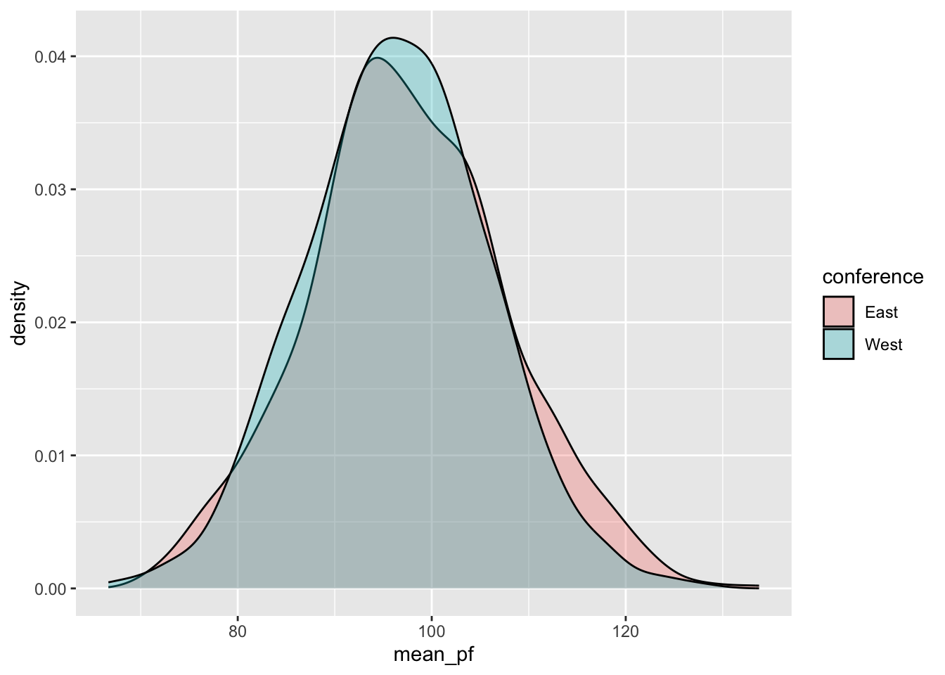
It’s pretty hard to tell if these are different, right?
So What? Using Percentiles of the Resampled Distribution
Now we can make some statements about uncertainty. Based on this, we can pretend to be all-powerful voyager across universes, and conclude that Eastern conference players commit more personal fouls.
The easiest way to do this is just to create a new variable that indicates whether the Eastern conference players had more personal fouls than the Western conference players in a given random sample. But currently, our data is organized in the “long” format, right?
bsRes## # A tibble: 2,000 × 3
## conference mean_pf bsInd
## <chr> <dbl> <int>
## 1 East 84.4 1000
## 2 West 86.9 1000
## 3 East 91.5 999
## 4 West 93.2 999
## 5 East 102. 998
## 6 West 94.3 998
## 7 East 112. 997
## 8 West 102. 997
## 9 East 113. 996
## 10 West 94.5 996
## # ℹ 1,990 more rowsWe want to convert it to the “wide” format, which means that each row is a random sample simulation, and we have one column for the Eastern conference personal fouls, and one column for the Western conference personal fouls.
Let’s create this using either spread() or pivot_wider().
# Spread approach
bsRes %>%
  spread(conference,mean_pf)
## # A tibble: 1,000 × 3
## bsInd East West
## <int> <dbl> <dbl>
## 1 1 112. 92.3
## 2 2 110. 92.5
## 3 3 85.9 104.
## 4 4 103. 93.2
## 5 5 93.5 79.5
## 6 6 94.2 98.0
## 7 7 93.8 94.1
## 8 8 94.6 89.9
## 9 9 91.8 79.8
## 10 10 92.0 101.
## # ℹ 990 more rows# Pivot-wider approach
bsRes %>%
pivot_wider(names_from = 'conference',values_from = 'mean_pf')## # A tibble: 1,000 × 3
## bsInd East West
## <int> <dbl> <dbl>
## 1 1000 84.4 86.9
## 2 999 91.5 93.2
## 3 998 102. 94.3
## 4 997 112. 102.
## 5 996 113. 94.5
## 6 995 117. 84.6
## 7 994 92.5 92.3
## 8 993 106. 98.1
## 9 992 101. 85.5
## 10 991 97.2 99.7
## # ℹ 990 more rowsWith the data organized in “wide” format, it is now trivial to calculate whether the Eastern players had more personal fouls than the Western players.
bsRes %>%
  pivot_wider(names_from = 'conference',values_from = 'mean_pf') %>%
  mutate(diff = East - West,
         EastMore = diff > 0)
## # A tibble: 1,000 × 5
## bsInd East West diff EastMore
## <int> <dbl> <dbl> <dbl> <lgl>
## 1 1000 84.4 86.9 -2.47 FALSE
## 2 999 91.5 93.2 -1.73 FALSE
## 3 998 102. 94.3 7.53 TRUE
## 4 997 112. 102. 9.75 TRUE
## 5 996 113. 94.5 18.3 TRUE
## 6 995 117. 84.6 32.8 TRUE
## 7 994 92.5 92.3 0.235 TRUE
## 8 993 106. 98.1 7.37 TRUE
## 9 992 101. 85.5 15.9 TRUE
## 10 991 97.2 99.7 -2.44 FALSE
## # ℹ 990 more rowsExpressing confidence
To express our “confidence” in the conclusion that Eastern conference players made more personal fouls than Western conference players in the 2018-2019 season, we can simply calculate the proportion of the 1,000 simulated alternate universes in which this conclusion was true! To do this, we just take the overall average of our new column EastMore!
bsRes %>%
  pivot_wider(names_from = 'conference',values_from = 'mean_pf') %>%
  mutate(diff = East - West,
         EastMore = diff > 0) %>%
  summarise(conf = mean(EastMore))
## # A tibble: 1 × 1
## conf
## <dbl>
## 1 0.5310.531. Or, approximately 53.1%. In other words, in the data, Eastern conference players committed more personal fouls in a little more than half of the 1,000 simulated realities.
How strong is our argument do you think? Typically social scientists adhere to a norm of at least 95% confidence before we feel comfortable defending our conclusion. Otherwise, how can we be certain that it’s not just a fluke of the data?
Try it yourself
Quick Exercise 2 How confident are you that Eastern conference players are better than Western conference players on each of these metrics?
- Turnovers
- Rebounds
- Field goals
# INSERT CODE HERE